Usage Guide
0. Data Preparation
To analyze your spatial proteomics datasets with C-COMPASS, you need the following input files: a fractionation dataset, a marker list, and, for some analyses, a total proteome dataset. These are described in detail below. There is also a sample dataset available.
Fractionation Data (required)
The fractionation dataset contains the protein amounts across different
fractions. This dataset is typically derived from a spectral search software,
such as MaxQuant, Spectronaut, DIANN, or others.
The data must be reported as a pivot report table, meaning that your table
includes one row per protein and one column per sample
(e.g., Condition1_Replicate1_Fraction1,
Condition1_Replicate1_Fraction2, and so on…).
The data is expected to be in a tab-delimited format (.txt or .tsv).
Fractionation data example table.¶ ProteinGroups
GeneName
Condition1_Replicate1_Fraction1
Condition1_Replicate1_Fraction2
P001
G001
0.45
0.78
P002
G002
0.67
0.34
P003
G003
0.89
0.56
P004
G004
0.12
0.91
The required columns are:
A unique protein identifier column (such as ProteinGroups, UniProtID, or similar)
Potentially a second identifier/key that is compatible with your marker list (usually the GeneName). Ensure that these keys exactly match the ones in your marker list.
Columns for each condition/fraction/replicate.
The table may also contain additional columns. You can remove them in C-COMPASS.
There are no restrictions on the column names or order. However, assigning the condition, replicate, and fractions metadata in C-COMPASS will be easier if the columns for the different fractions of a given condition/replicate are grouped together, and the order of the columns is consistent across replicates and conditions. The number of fractions may differ across replicates.
Note
You should not apply any data processing before loading the dataset in C-COMPASS.
If you have a dataset that is already pre-processed, please make sure that the data still fulfill the following requirements:
Any normalization must conserve the intensity ratios between fractions. That means, a 0-1 MinMax scaling or area-based scaling is ok, but do not apply any log-transformation.
A normalization that corrects values across different replicates or conditions is ok as long as the integrity of the profiles per replicate are conserved.
C-COMPASS was optimized on LFQ values but other quantities like TMT can also be used. Different conditions or different replicates can derive from several experiments/runs as long as the identifiers are compatible, but each replicate fractionation must derive from the same analysis file.
Marker List (necessary)
A list of marker proteins is required to train the neural network model. This list should contain proteins that are known to be localized to specific compartments. The marker list can be derived from previous publications or databases relevant to your project.
The data is expected to be in a tab-delimited format (.txt or .tsv).
The table must contain at least two columns:
An identifier/key compatible with the key column in the fractionation dataset, usually the GeneName
A compartment annotation column that specifies on which in compartment the each protein are located
GeneName |
Compartment |
|---|---|
G001 |
ER |
G002 |
Golgi |
G003 |
Mitochondria |
Multiple files can be combined in C-COMPASS and compartments can be renamed or excluded.
Total Proteome Data (optional)
Total proteome data is only necessary for normalization of relocalization events to study the abundance change inside compartments across conditions (referred to as class-centric changes in the GUI).
The data is expected to be in a tab-delimited format (.txt or .tsv).
Data must be presented as a ‘pivot report table’ That means, you need one
column for each of your samples (e.g. TP_Condition1_Replicate1,
TP_Condition1_Replicate2, and so on…).
Table must contain the same unique identifier column that was used for the fractionation file (ProteinGroups, UniProtID or similar).
Total Proteome data example table¶ ProteinGroups
TP_Condition1_Replicate1
TP_Condition1_Replicate2
P001
0.45
0.78
P002
0.67
0.34
P003
0.89
0.56
P004
0.12
0.91
The table can also contain additional columns that are not necessary. You can remove them in C-COMPASS. Total Proteome data should derive from the same experiment to be comparable.
Additional Notes
If using an export file from Perseus, ensure that the file does not contain a second-layer header.
Input datasets (for both fractionation and total proteome) can be stored in the same file or split across different files. If they are split, ensure that the identifiers are consistent.
Sample Data
Sample data files with artificial data are available for download at
![]() .
.
Computation time for this dataset using a single core on a standard desktop computer:
Preprocessing of Gradient and TotalProteome Data takes only up to a few minutes.
Neural Network training for a dataset with three conditions and four replicates takes around 1-2h.
Calculation of static predictions (per condition) takes a few minutes.
Calculation of conditional comparisons (global comparison) takes up to 30min.
Calculation of class-centric statistics and comparison takes up to 10 min.
1. Graphical User Interface (GUI)
C-COMPASS allows you to save and load your sessions via the main menu (). Saving after each significant step is recommended to avoid data loss. The session file, which includes all datasets, marker lists, settings, analyses, trainings, and statistics. These will be fully restored upon loading ().
There are currently two options for saving your session:
A NumPy/pickle (
.npy) file. This is the fastest option. However, those files will not necessarily work across different versions of Python, C-COMPASS, numpy, or pandas.A zip (
.ccompass) file. This is significantly slower but more reliable across different versions.
The format can be chosen in the save dialog.
2. Before training
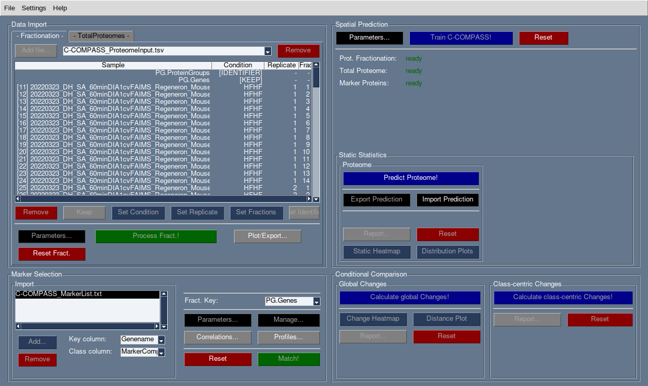
Data Import
There are two tabs for data import: Fractionation and TotalProteome.
Fractionation data can be analyzed independently, but TotalProteome is required for final class-centric statistics.
Use the Add file… button to import datasets. Multiple datasets can be imported and will appear in the dropdown menu. To remove a dataset, select it from the dropdown and click Remove.
The table will display all column names found in the selected dataset.
Sample Annotation
For Fractionation data: Assign the condition, replicate number, and fraction numbers by selecting the relevant column names and clicking the appropriate button.
For TotalProteome data: Follow the same steps as Fractionation data, using consistent condition names.
Set the identifier column (e.g., ProteinGroups) for both Fractionation and TotalProteome datasets using the Set Identifier button. Ensure compatibility between these columns.
For other columns, either remove them or mark them as Keep. Data marked as Keep will not be used in the analysis but will be available for export.
IMPORTANT: Ensure that the column matching the marker list’s naming (usually the gene name column) is kept.
Pre-Processing
Once columns are annotated, click Process Fract. or Process TP to import the data.
Fractionation and TotalProteome data can be processed independently.
Marker List Import
In the Marker Selection frame, load marker lists via the Add… button. Multiple marker lists can be imported, and individual lists can be removed using the Remove button.
Imported marker lists will be displayed in the box.
For each marker list, specify the key column (e.g., gene names) and the class column (e.g., compartment).
In the Fract. Key section, select the column from the fractionation dataset that contains the compatible key naming. If the identifier and key column are the same, select [IDENTIFIER].
Marker Check & Matching
Click Manage… to view all class annotations from the marker lists. Unselect any classes you do not want in the analysis or rename them.
Classes with different nomenclatures (e.g.,
ERvs.Endoplasmic Reticulum) can be merged by giving them the same name.Median profiles of marker proteins and Pearson correlation matrices can be displayed via the corresponding buttons. Export options for plots and tables are available.
Confirm your marker selection by clicking Match!.
3. Training
Start the training process by clicking Train C-COMPASS.
Various network architectures will be trained and evaluated for optimal results. This process may take over an hour, depending on dataset size. By default, training is performed on a single core, but you can change this via .
Progress will be shown in the progress dialog and more details are shown on the background console window.
Hint: Save your session after training to avoid repeating the process.
4. After training
Statistics
After training, create Static Statistics via Predict Proteome to generate quantitative classifications for each condition.
Predictions can be exported or imported for comparison across sessions, ensuring compatible identifiers.
Use the Report button to export results.
Create simple plots and export them, along with the corresponding data tables.
Conditional Comparison - Global Changes
- Calculate Global Changes compares localization across
conditions, providing relocalization results.
Results can be displayed and exported similarly to the statistics.
Conditional Comparison - Class-centric Changes
Calculate Class-Centric Changes provides detailed statistics on protein relocalization within compartments across conditions:
CPA (Class-centric Protein Amount): The amount of protein within a compartment, normalized by total proteome data. This is a relative value that requires comparison across conditions.
CFC (Class-centric Fold-Change): The fold change of proteins across conditions within a compartment, based on CPA values. Only proteins with valid fractionation and total proteome data for both conditions will have CFC values.
5. Spatial Lipidomics
C-COMPASS has been used for spatial lipidomics analysis, though no dedicated feature currently exists for multi-omics analysis.
You can concatenate proteomics and lipidomics datasets into one file before importing into C-COMPASS. Lipids will be treated like proteins, and spatial information can be derived similarly. Future versions of C-COMPASS will include features specifically designed for lipidomics.
6. Parameters
All parameters are set to default values used in our publication. It is not recommended to change them unless you are familiar with the procedure and its impact on results.
Fractionation Data Parameters
Parameters for analysis and visualization can be adjusted independently.
- Min. valid fractions:
Profiles with fewer valid values across fractions can be filtered out.
- Found in at least X Replicates:
Proteins found in fewer replicates than specified will be removed.
- Pre-scaling:
Options include MinMax scaling or Area scaling.
- Exclude Proteins from Worst Correlated Replicate:
Removes the replicate with the lowest Pearson correlation.
- Post-scaling:
Same options as Pre-scaling, useful for median profiles.
- Remove Baseline Profiles:
Removes profiles with only 0 values after processing.
TotalProteome Parameters
- Found in at least X:
Similar to Fractionation data, this filters proteins found in fewer replicates.
- Imputation:
Missing values can be replaced by 0 or other values.
Marker Selection Parameters
Discrepancies across marker lists can be handled by excluding markers or taking the majority annotation.
Spatial Prediction Parameters
WARNING: Changes here are not recommended!
Various upsampling, noise, and SVM filtering methods are available for marker prediction.
Other parameters for network training and optimization can be configured, including dense layer activation, output activation, loss function, optimizers, and number of epochs.